Speeding Up Transformer Inference
02/2023 - Philip
Recently I’ve been playing around with Transformer models on a GPU with the goal of optimizing the inference of the model.
The rising interest in real applications of large language models (and deep learning models) is met with the practical limitations of economics and compute.
One of the drivers of deep learning is faster GPUs through Moore’s law which has been a several decades long tailwind. The other way of progressing deep learning is to figure out how to do “more with less”. My sense is that we are still in early stages of improving and designing transformer models for inference.
The task to do “more with less” is not easy, however. Transformer language models are autoregressive meaning more computations will depend on each other sequentially, and many of the SoTA models are absurdly large. The autoregressive nature also means there are many components of the model that are dynamic in shape, making them harder to optimize on the CUDA graph level.
In this post I will be primarily concerned with implementing various optimizations for the inference part of transformer models1. Perhaps in another post I can explore ways to optimize training more with less.
Benchmark
Hardware:
- \(1\times\)
NVIDIA T4(16GB GPU memory) - GCP
n1-standard-4(15GB host memory and 4 vCPUs)
As a benchmark, I will generate up to 300 tokens given a prompt. For the prompt I’ll use a passage from Lisp developer Richard P. Gabriel in his essay “The Rise of Worse is Better”:
Early Unix and C are examples of the use of this school of design, and I will call the use of this design strategy the New Jersey approach. I have intentionally caricatured the worse-is-better philosophy to convince you that it is obviously a bad philosophy and that the New Jersey approach is a bad approach. However, I believe that worse-is-better, even in its strawman form, has better survival characteristics than the-right-thing, and that the New Jersey approach when used for software is a better approach than the MIT approach.
Let me start out by retelling a story that shows that the MIT/New-Jersey distinction is valid and that proponents of each philosophy actually believe their philosophy is better.
Two famous people, one from MIT and another from Berkeley (but working on Unix) once met to discuss operating system issues. The person from MIT was knowledgeable about ITS (the MIT AI Lab operating system) and had been reading the Unix sources. He was interested in how Unix solved the PC loser-ing problem. The PC loser-ing problem occurs when a user program invokes a system routine to perform a lengthy operation that might have significant state, such as IO buffers. If an interrupt occurs during the operation, the state of the user program must be saved. Because the invocation of the system routine is usually a single instruction, the PC of the user program does not adequately capture the state of the process. The system routine must either back out or press forward. The right thing is to back out and restore the user program PC to the instruction that invoked the system routine so that resumption of the user program after the interrupt, for example, re-enters the system routine. It is called PC loser-ing because the PC is being coerced into loser mode, where loser is the affectionate name for user at MIT.
When using the OpenAI BPE tokenizer the prompt results in 374 tokens.
The Model
I’m using the GPT2 model from OpenAI on Hugginsface which as a total of 125M parameters.
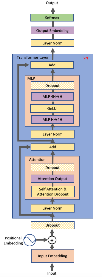
I think it will be useful to map out this model (which is going to be more or less consistent with GPT3 or other LLM transformer variants). The GPT architecture looks something like this:
 |
|---|
| Transformer diagram. Source: Megatron-LM paper |
Note that for the architecture is still pretty similar to the one used in the All you need is Attention paper. Some of the key changes are:
- Layer norm is moved to before the Multi-Head Attention instead of after which supposedly helps with gradient stability during training.
- As we’re doing language generation, the encoder-decoder setup becomes a singular encoder that is applied autoregressively to its outputs.
- The \(QK^T\) matrix is masked to become lower triangular to maintain autoregressive properties. Considering that \(Q=[q_0,\ldots,q_T]\) (rows) and \(K^T=[k_0;\ldots;k_T]\) (columns), masking \(QK^T\) means we only consider attention dot products for \(q_i\cdot k_j\) when \(j\leq i\).
As an aside, I think it is rather interesting that the architecture has not changed much for the past 5 years. It seems though that there is still a lot of room for developing architectures that might be more specifically designed for fast inference. A few ideas here, but perhaps for another day.
For convenience I am using Andrey Karpathy’s nanoGPT repo as a boilerplate. Implementing a basic base model itself is rather straightforward. Describing the key modules from the top down:
class GPT(nn.Module):
"""
idx -> x (embedding) -> x: block_1(x) -> x: block_2(x) -> ... -> x: block_n_layer(x) -> x: layer_norm(x) -> logits
"""
class Block(nn.Module):
"""
x -> x: layer_norm(x) -> x: x + CausalSelfAttention(x) -> x: layer_norm(x) -> x: x + MLP(x)
"""
class CausalSelfAttention(nn.Module):
"""
x -> Q, K, V: xW_Q, xW_K, xW_V -> y: proj(softmax(QK^T/sqrt(d_m))V)
"""
Enumerating the computations on the model from the ground up (I’m going to ignore a lot of asymptotically smaller components like bias or softmax):
- Input \(x\) is a tensor of shape \(\mathbb{R}^{B\times T\times C}\) where \(B=1\) is the size of the batch, \(T\leq1024\) is the sequence length and \(C=768\) is the embedding dimensionality
CausalSelfAttention():- Inputs \(x\) and multiples by three matrices of shape \(\mathbb{R}^{C\times C}\) to obtain \(n_h\) sets of \(Q, K, V\in\mathbb{R}^{B\times T\times n_h\times C/n_h}\) where \(n_h=12\) is the number of heads.
- Compute \(\text{softmax}(QK^T/\sqrt{C/n_h}) V.\) Then project multiplying a matrix of size \(\mathbb{R}^{C\times C}\).
- In our case the FLOPs of one CausalSelfAttention becomes \(4TC^2+2CT^2=4026531840\approx4.0\) GFLOPs.
MLP():- Inputs \(x\) and applies a linear projection of dimension \(\mathbb{R}^{C\times 4C}\) followed by GeLU nonlinearity and another projection of shape \(\mathbb{R}^{4C\times C}\)
- The FLOPs of one MLP becomes \(8TC^2=4831838208=4.83\) GFLOPs.
Block():- Takes \(x\in\mathbb{R}^{B\times T\times C}\) and applies layer norm,
CausalSelfAttention(), self addition, another layer norm, aMLP(), and another self addition. - The attention and the multilayer perception result in a total of \(4.0+4.83=8.83\) GFLOPs.
- Takes \(x\in\mathbb{R}^{B\times T\times C}\) and applies layer norm,
GPT():- For \(n_{layer}=12\) times apply:
x = block_i(x)
- Apply layer norm to \(x\)
- Finally project \(x\) by multiplying with a matrix of shape \(\mathbb{R}^{C\times n_V}\) where \(n_V=50257\) is the vocab size.
- The 12 blocks result in \(12*8.83=105.96 GFLOPs\) and the final projection results in \(TCn_v=39523713024=39.5\) GFLOPs (it’s actually 1024 times less than this at inference because we’re only interested in the final logit). So in total we are working with at least \(\fbox{145.46}\) GFLOPs.
- For \(n_{layer}=12\) times apply:
One can estimate the FLOPs using the following script:
"""
Approximates flops, only matmuls.
"""
def compute_FLOPs(config, B=1, T=1024):
    flops_dict = {}
    C = config.n_embd
    hs = C // config.n_head
    #Causal Self Attention: xW_Q, xW_K, xW_V, QK^TV, c_proj
    flops_dict["attention"] = B*(4*T*C*C+2*T*T*C)*config.n_layer
    #MLP
    flops_dict["mlp"] = B*(4*T*C*C+4*T*C*C)*config.n_layer
    #lm_head
    flops_dict["lm_head"] = B*(T*C*config.vocab_size)
    print(flops_dict)
Running this for a few values we can get a table of FLOPs breakdown across models for a single inference step for a context window of 1024 tokens and a batch size of 1:
| Model | Attention | MLP | LM Head | Total |
|---|---|---|---|---|
| GPT2 125M | \(4.8\times10^{10}\) (33.1%) | \(5.8\times10^{10}\) (39.8%) | \(4.0\times10^{10}\) (27.1%) | \(1.5\times10^{11}\) |
| GPT2-medium 350M | \(1.5\times10^{11}\) (37.4%) | \(2.1\times10^{11}\) (49.9%) | \(5.3\times10^{10}\) (12.7%) | \(4.1\times10^{11}\) |
| GPT2-large 774M | \(3.38\times10^{11}\) (38.1%) | \(4.8\times10^{11}\) (54.5%) | \(6.6\times10^{10}\) (7.4%) | \(8.9\times10^{11}\) |
| GPT2-xl 1.56B | \(6.6\times10^{11}\) (37.9%) | \(1.0\times10^{12}\) (57.4%) | \(8.2\times10^{10}\) (4.7%) | \(1.8\times10^{12}\) |
| GPT-3 175B | \(6.2\times10^{13}\) (34.1%) | \(1.2\times10^{14}\) (65.5%) | \(6.3\times10^{11}\) (0.3%) | \(1.8\times10^{14}\) |
Note how as the model gets deeper, the attention and MLP components become a much larger portion of the total FLOPs. This is because the lm_head only scales linearly with \(T\) and \(C\) whereas the MLP scales quadratically with embedding size and the attention scales quadratically with both embedding size and context length. Both the MLP and attention scale linearly with the number of layers as well.
Our NVIDIA T4 is able to do 8.1 TFLOPs of FP32 and 65 TFLOPs of FP16. If we could magically do all the computations of our model at once, this would mean we could do a single step in around 2 ms on FP16. Note however that this is not going to be attainable since many of these computations depend on each other and cannot be parallelized. Furthermore there are also memory and overhead latencies to consider
With no changes, our experiment generating 300 steps results in an average of 24 ms per step or a total of 7.27 s.
Optimization 1: KV Cache
One problem with our vanilla GPT model is that we are doing a lot of redundant computations as we autoregressively apply steps for a particular sequence. For instance, consider that at time \(T-1\) we compute \(QK^T\) where \(Q=\left[\begin{array}{c}q_1 \\\vdots \\q_{T-1}\end{array}\right]\) and \(K^T=\left[\begin{array}{ccc}k_1 & \cdots & k_{T-1}\end{array}\right]\) which results in the matrices:
\[\begin{align*} \text{step }(T-1)&: \text{mask}(QK^T) = \left[\begin{array}{ccc}q_1\cdot k_1 & \cdots & 0 \\\vdots & \ddots & \vdots \\q_{T-1}\cdot k_1 & \cdots & q_{T-1}\cdot k_{T-1}\end{array}\right]\\ \text{step }(T)&: \text{mask}(QK^T) =\left[\begin{array}{cccc}q_1\cdot k_1 & \cdots & 0 & 0 \\\vdots & \ddots & \vdots & \vdots \\q_{T-1}\cdot k_1 & \cdots & q_{T-1}\cdot k_{T-1} & 0 \\q_T\cdot k_1 & \cdots & q_T\cdot k_{T-1} & q_T\cdot k_T\end{array}\right] \end{align*}\]One can see that when we want to compute the step at time \(T,\) \(\text{mask}(QK^T)\) has exact same entries as before but with one additional row and column. Because the lower triangular property of this matrix, we only need to compute a single row of size \(T\) as the additional column will be all zeros except the last entry which will be included in the row we append.
In of itself, saving \(QK^T\) computations from previous steps doesn’t help us that much since in total we only have around \(12\times T^2\times 64=805306368=.8\) GFLOPs of this computation (although note this will be more significant for deeper models). In fact, when I first just modified the model to save \(QK^T\) while appending the a single row I didn’t notice any performance gains.
The useful insight here is that not only do we just need to compute the bottom row of the attention matrix, we can actually use this to only compute most of the rest of the model (MLP and lm_head) on a single vector input \(T=1.\) One can see after examining the how the components of the attention matrix change from step \(T-1\) to step \(T\) the following:
- \(\text{softmax}(QK^T/\sqrt{C/d_h})V\) does not change aside from the bottom row which is given by \(\text{softmax}(q_TK/\sqrt{C/d_h})V.\) The \(V\) multiplication doesn’t change matrix across steps because of the lower triangular nature of the matrix.
- \(K\) and \(V\) do not change either aside from appending \(x_TW_K\) and \(x_TV_K\) as the bottom rows of both, respectively.
One can also see that as we pass our attention matrix to the subsequent layers (MLP or last projection) that the only row that changes and matters is the bottom row. In the last projection we take this bottom row and project it onto a vector of size \(n_V\) which acts as logits for our set of possible output tokens.
This means that once we have \(K\) and \(V\) cached from a previous step, we only need to run parts of the model computations for an input with \(T=1.\) In the case of the MLP this means the \(8TC^2\) becomes \(8C^2=.004\) GFLOPs and the final projection only requires \(39.5/1024=.039\) GFLOPs. The bottom attention row is going to only be around \(2\times n_h\times T=24576\) FLOPs which is negligible. So roughly we have a total around \(.5\) GFLOPs if we cached \(K\) and \(V\) (almost a 300x reduction of FLOPs). Note however our worst case is the same as before which will occur on cold start (e.g. you start by prompting with more than 1024 tokens).
Implementing KV cache was rather straightforward. For each module in the vanilla model I create a child class along with a flag that indicates whether we are running assuming a cache or not. If cached=False it’s business as usual but when cached=True we run the optimized version:
class KVCausalSelfAttention(CausalSelfAttention):
def **init**(self, config):
super().**init**(config)
self.register_buffer("K_cache", torch.zeros(64,config.n_head, config.block_size, config.n_embd // config.n_head))
self.register_buffer("V_cache", torch.zeros(64,config.n_head, config.block_size, config.n_embd // config.n_head))

    def forward(self, x, cached=False):
        (
            B,
            T,
            C,
        ) = x.size()  # batch size, sequence length, embedding dimensionality (n_embd)

        if not cached:
            q, k, v = self.c_attn(x).split(self.n_embd, dim=2)
            k = k.view(B, T, self.n_head, C // self.n_head).transpose(
                1, 2
            )  # (B, nh, T, hs)
            q = q.view(B, T, self.n_head, C // self.n_head).transpose(
                1, 2
            )  # (B, nh, T, hs)
            v = v.view(B, T, self.n_head, C // self.n_head).transpose(
                1, 2
            )  # (B, nh, T, hs)
            self.K_cache[:B, :, :T, :] = k[:, :, :, :]
            self.V_cache[:B, :, :T, :] = v[:, :, :, :]
        if cached:
            q_T, k_T, v_T = self.c_attn(torch.unsqueeze(x[:, -1, :], dim=1)).split(
                self.n_embd, dim=2
            )
            q_T = q_T.view(B, 1, self.n_head, C // self.n_head).transpose(
                1, 2
            )  # (B, nh, 1, hs)
            k_T = k_T.view(B, 1, self.n_head, C // self.n_head).transpose(1, 2)
            v_T = v_T.view(B, 1, self.n_head, C // self.n_head).transpose(1, 2)
            self.K_cache[:B, :, :T, :] = torch.cat((self.K_cache[:B, :, :(T-1), :], k_T), dim=2)[:, :, -(T - 1) :, :]
            self.V_cache[:B, :, :T, :] = torch.cat((self.V_cache[:B, :, :(T-1), :], v_T), dim=2)[:, :, -(T - 1) :, :]
            att = F.softmax(
                (
                    (q_T @ self.K_cache[:B, :, :T, :].transpose(-2, -1))
                    * (1.0 / math.sqrt(self.K_cache[:B , :, :T, :].size(-1)))
                ),
                dim=-1,
            )
        else:
            att = (q @ k.transpose(-2, -1)) * (1.0 / math.sqrt(k.size(-1)))
            att = att.masked_fill(self.bias[:, :, :T, :T] == 0, float("-inf"))
            att = F.softmax(att, dim=-1)
        att = self.attn_dropout(att)
        y = att @ self.V_cache[:B, :, :T, :]
        y = y.transpose(1, 2).contiguous().view(B, T, C)
        y = self.resid_dropout(self.c_proj(y))
        return y
Given these changes, on an NVIDIA T4 our experiment generating 300 steps now averages around 10 ms per step or a total of 3.0 s. This is a huge speedup from our original 24 ms per step and we didn’t even have to make any assumptions about the hardware. In fact, I was developing and testing much of the code on my MacBook Pro that has a 16GB M1 Chip (no NVIDIA GPU). Since my MacBook Pro is going to be grossly compute bound, I get even more exaggerated results. My MacBook takes around 360 ms per step or a total of ~108 s for the vanilla transformer. With KV Caching my laptop does 27ms per step for a total 8.10 s (almost as fast as uncached model on NVIDIA T4!).
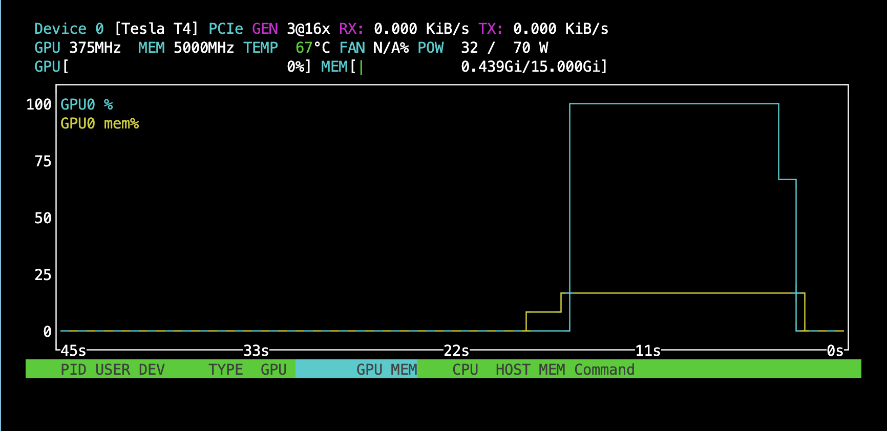
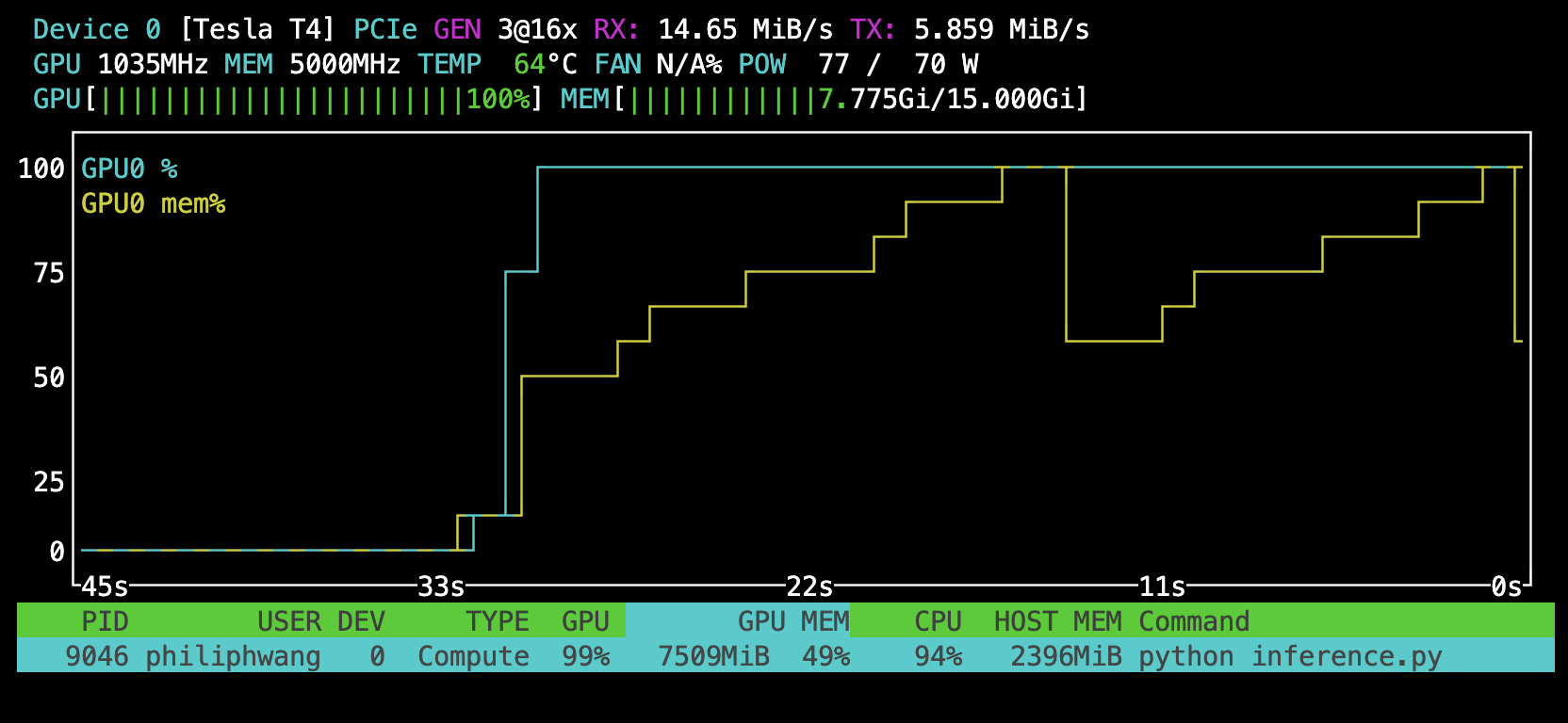
Doing this optimization reduces the flops so much that we seem to no longer be as compute bound before (suggesting the latencies due to memory and overhead are now more significant):
 |
|---|
 |
| Top: No KV caching (compute bottlenecked). Bottom: KV caching (much lower GPU utilization) |
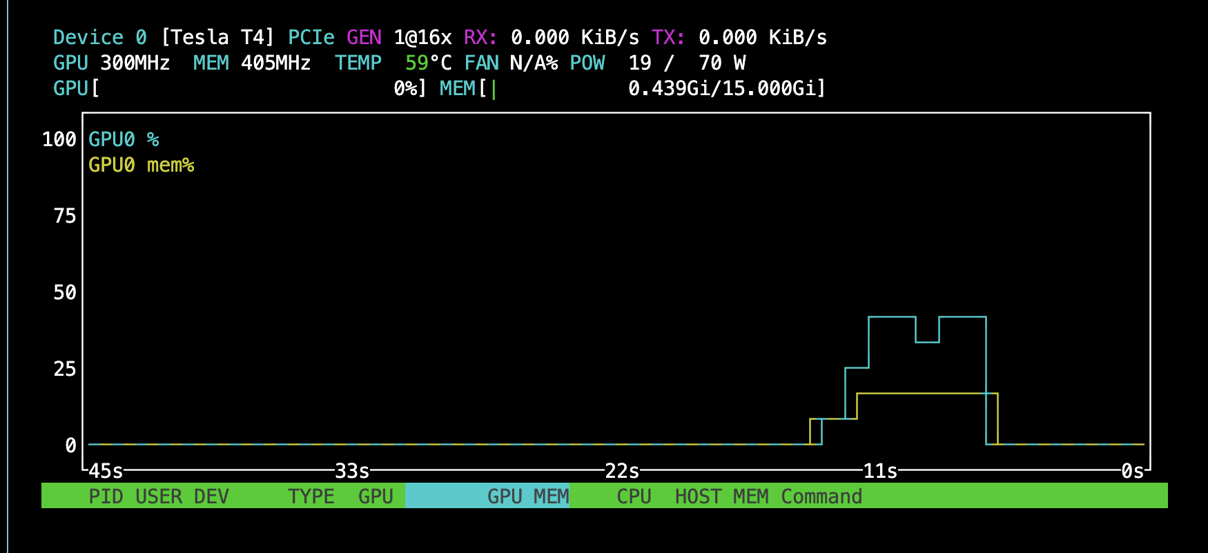
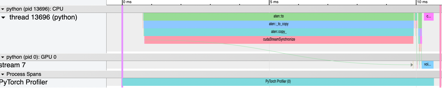
I can confirm I am CPU bound by using torch profiler:
 |
|---|
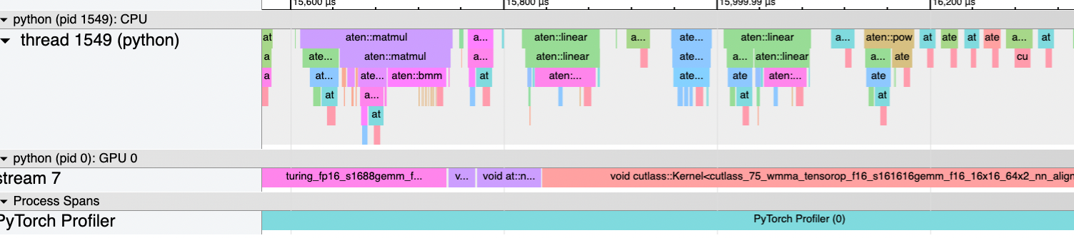 |
| Top: With KV caching we are CPU bound (large gaps on GPU stream indicate GPU is waiting on CPU) Bottom: With no KV caching the GPU is still occupied much of the time. |
One issue with the KV cache is that it requires a lot of space to store. The total storage space in terms of number of number of floating points will be \(2BTCn_\text{layer}\) For GPT-xl this means a batch of 512 and a context window of 1024 might need to cache 322GB (assuming 4 byte floating points). For GPT3 with a context window of 2048 this value becomes 9.9TBs (around 20GBs per individual) which is an order of magnitude larger than the model size.
These numbers become important to consider in the context of user-facing services. Consider that there are significant transfer latencies from cold storage to memory to GPU memory for these cached values (in addition to storage and transfer costs for cloud services). There are further complications to consider given the GPU’s VRAM will cap the amount of cached values one can keep on-chip at the same time.
Let’s assume we have a Nvidia DGX-2 GPU which has a total of 512GB of VRAM. To make things easier let’s also assume we have figured out how to run GPT3 on fp8 for all parameters and that we have already loaded the entire 135GB model onto VRAM. That means a single DGX-2 will be able to store the largest KV caches of at most a batch of size \(\lfloor(512-135)/20\rfloor=18\) at a time (ignoring that we also have intermediate writes to VRAM during computation). NVIDIA claims the DGX-2 can load up to 200GB/s from local drives meaning it would take around 1.8 seconds to load the KV caches into VRAM (this can probably be absorbed asynchronously with a nice login animation). Let’s assume that all 18 people occupy this machine for an entire hour (this is very generous in practice). 16 V100 16GB (DGX-2 uses 32GB) would cost around $8.80/hr on Lambda Labs. This would mean it would cost us around $0.49 to serve each customer for an hour assuming we stored the worst case KV cache.
I’m not claiming this is exactly what companies servicing transformer’s on APIs are dealing with exactly (they might be using a smaller model, they could be using a better hardware setup, the context window might be smaller, maybe we don’t need to cache that aggressively etc.), but the point here is to illustrate that using the KV cache involves a number of economic and engineering complexities to consider.
Obviously whether you even use the KV cache depends on the specific use case you want to serve. I could see a case where one prefers to serve a large batch of invocations at once rather than minimizing latency. Furthermore, there could be other changes one could make like offloading the KV cache until needed into CPU memory at the expense of memory transfer latency.
Optimization 2: FP16
Given the memory issues KV might cause, one optimization we can make invovles changing the numerical data type used by the GPU.
By setting dtype='float16' instead of float32 we should be able to use half the memory as before. For a batch size of 1 using the KV cache I don’t notice any significant changes in performance. However, when I increase the batch size I start to see stark differences.
When I use a batch size of 256 with the KV cache on float32 I run out of memory:
torch.cuda.OutOfMemoryError: CUDA out of memory. Tried to allocate 1.10 GiB (GPU 0; 14.56 GiB total capacity; 11.48 GiB already allocated; 162.44 MiB free; 13.62 GiB reserved in total by PyTorch) If reserved memory is >> allocated memory try setting max_split_size_mb to avoid fragmentation. See documentation for Memory Management and PYTORCH_CUDA_ALLOC_CONF.
For a batch of 256 on float16, however, I am able to complete the task in a total of 43.1s or 144ms per step. So in the extreme case, float32 occupies too much space in the KV cache to complete but float16 doesn’t. Note that in float32 each number is 4 bytes and we have up to \(768\times12\times1024\times256\times4=9.7\times10^9\) bytes or 9.7 GB to store. Combined with our model size and the intermediate computation states stored on memory, using float32 eventually makes our GPU OOM.
Furthermore, in addition to being able to run larger batches we seem to also get latency benefits for larger batches:
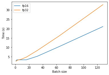 |
|---|
Latency gap across fp16 and fp32 using the KV cache. By the way, since I’m lazy I’m not doing enough samples to be able to give you confidence intervals. |
One explanation for why this gap exists at larger batches but not at smaller is that the numerical type starts to matter the more compute bound we are. Remember how when KV caching for a batch size of 1 the GPU was idly waiting much of the time on the CPU. When I use a batch size of 1 but don’t use the KV cache, we reach 100% GPU utilization for both fp16 and fp32 and fp16 is significantly faster by 6 seconds. Note that the NVIDIA claims the T4 is able to do fp16 at 65.1 TFLOPs and fp32 at 8.1 TFLOPs
 |
|---|
Batch size of 64 for fp32. |
Optimization 3: Vocab size
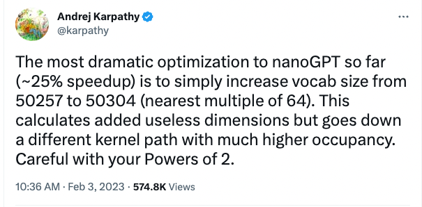 |
|---|
| Andrej Karpathy had a tweet that claims a large speed up comes from changing the vocab size to a multiple of 64. |
Now I will test changing the vocab size from 50257 to 50304 (nearest multiple of 64).
When I implemented this for inference I didn’t get any improvements. This is most likely because towards the end of the model, the lm_head projection actually accounts for very few FLOPs (we only multiply the last logit meaning this accounts for .04 GFLOPs) and we are not GPU bottlenecked (most of the memory overhead does not involve intra-GPU transfer):
 |
|---|
Trace of the last projection. The projection multiplication is the last block in blue in the GPU section (less than 1ms). GPU is waiting a lot towards the end, and the projection computation is very small. |
However, I start to see a difference during training (where we multiply all \(T\) logits by the lm_head weights). When I use a batch size of 2 with 32 gradient accumulation microsteps for 30 iterations I see around a 10% improvement in speed when using the larger vocab size that’s divisible by 64. The 50304 vocab size averaged around 8595.36ms per iteration and the 50257 vocab size averaged around 9205.20. The sample standard deviation of both were around 50ms so after doing a Student’s t-test I find the P-value is less than 0.0001. Therefore it is highly unlikely there is no difference made here between the two vocab sizes.
Why might we expect this seemingly arbitrary change improve performance? I prefer not to cargo cult this change as some “powers of 2” glitch. I think the explanation does not have to be as esoteric when we think about what might be going on at the systems level.
GPUs have various physical properties that must be considered when reducing the number of sequential operations. I came across a great explanation for what’s going on this thread. Much of the performance hit is because dimensions of the matrix that are cleanly divisible by the cache line of the GPU will be able to load elements at once whereas those that are not cleanly divisible might have to make sequential loads from cache to read an element2. The other performance discontinuity can come from the fact we have a limited number of stream multiprocessors (SMs; which constitute a unit of a collection of cores on the GPU). When the matrix is large enough, we will have to have the SMs perform computations in waves. Each wave can have the SMs perform computations simultaneously, but when we are done with a wave, if there is still leftover computation we need to launch another wave (even if the leftover is small).
At a high level, the more we can parallelize operations and more efficiently use faster memory components, the better. While we are typically working with simpler abstractions at the application layer, utilizing the GPU properly requires us to be aware of how inefficiencies might arise from what’s happening mechanically on the systems level of the GPU.
The impact of dimension multiples on cuBLAS is confirmed by NVIDIA:
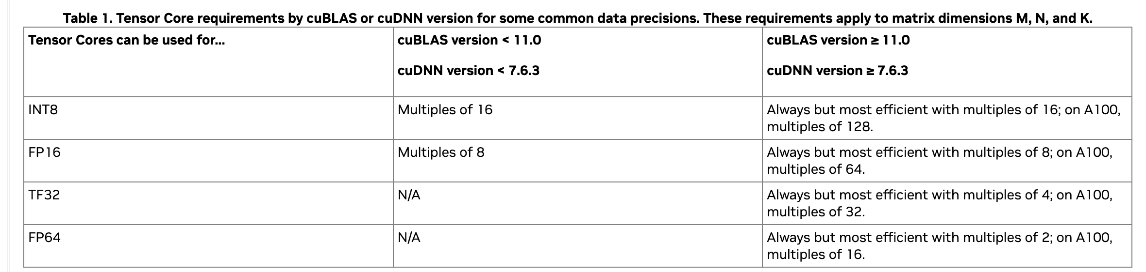 |
|---|
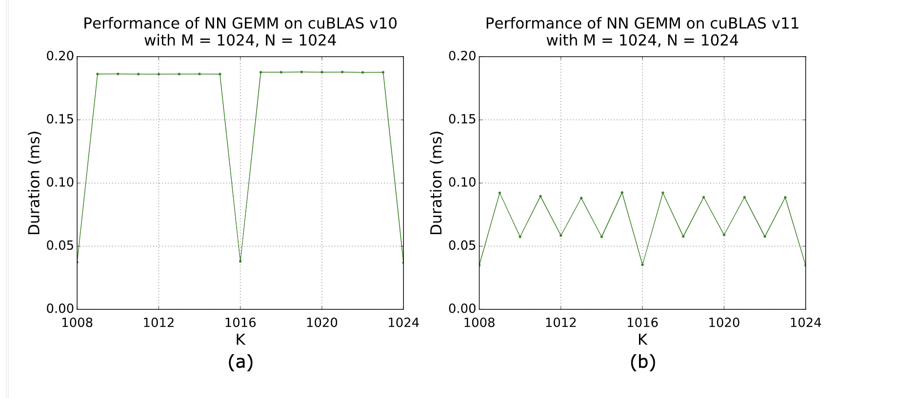 |
| From the NVIDIA developer guide which confirms performance changes as the dimension modulo 64 changes. |
Optimization 4: CPU Overhead
Recall how we were very CPU bound when using the KV cache:
|
|---|
| With KV caching we are CPU bound (large gaps on GPU stream indicate GPU is waiting on CPU) |
Before each GPU kernel is run, it is first launched by the CPU through PyTorch via Python then C++ then finally the underlying CUDA kernel to the GPU. This long execution path contributes overhead, especially when each GPU operation finishes very quickly. This is what causes the gaps where the GPU is waiting; the CPU is running slower than the actual GPU work3.
When running in PyTorch eager mode (normal PyTorch), this long execution path is repeated for each different input. The idea behind torch.compile is to “trace and compile” this execution path for the first input, and to cache a graph of this path for future inputs on the same model thereby reducing the CPU overhead.
Instead of paying the overhead at each kernel run, we can try to do the overhead work of multiple kernels at once. Building the graph that does this at the beginning will cause some latency at the beginning but ultimately amortize much of the overhead over each future iteration:
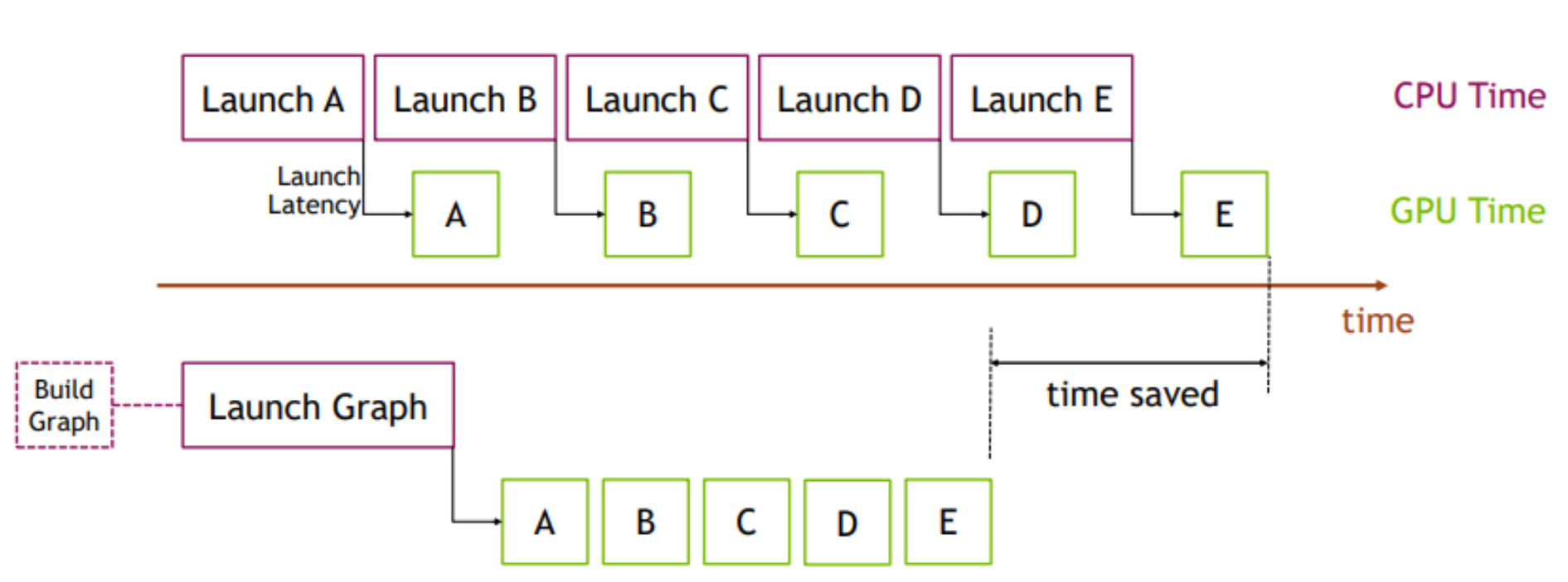 |
|---|
| Source: PyTorch Blog |
When I use torch.compile on mode="reduce-overhead" (which apparently does some CUDA graph level optimizations), instead of the 10ms per step from before, I am now able to consistently achieve 5ms per step. Note that I needed to do some amount of refactoring of my code to make this work. torch.compile seemed to work better when I fixed the size of the forward pass for example (this doesn’t effect us because when using the KV cache we only care about the last input token).
I still see a lot of GPU waiting when I examine the trace of a step. I’m guessing theoretically if I were to go a bit lower level we could speed this up much lower than 5ms.
Optimization 5: Things to try out (TODO)
There are a few other things but some these are a bit more involved to implement. Namely, int8 quantization, pruning, and flash attention kernel. Another optimization would be to use a sparser attention matrix and potentially using a kernel that only multiplies necessary values instead of computing the entire matrix. I haven’t done these yet, but I might if I have more time.
Acknowledgments
As I am his roommate, a lot of this project benefited from various conversations with Eric Wang who is financially ruined after buying a NVIDIA RTX 4090 recently.
-
Lilian Weng has a great literature review of inference related optimizations here ↩
-
I liked playing around with some matmul kernels and thinking about some of the boundary cases one would need to implement when the matrix dimensions are not evenly divisible by tile dimensions. It helped my understanding by reimplementing some of the kernels described by Simon Boehm. When the matrix is not evenly divided by tile dimensions, the edge cases can be somewhat tedious. ↩
-
Please read Horace He’s piece on compute, memory, and overhead latency if you have the time. ↩